Inall Polynomial Functions Are Continuous and Reline
Learning Objectives
-
- Introduction to polynomial functions
- Identify polynomial functions
- Identify the degree and leading coefficient of a polynomial function
- Algebra of Polynomial Functions
- Add and subtract polynomial functions
- Multiply and divide polynomial functions
- Composite and Inverse Functions
- Define a composite function
- Define an inverse function
- Use compositions of functions to verify inverses algebraically
- Identify an inverse algebraically
- Identify the domain and range of inverse functions with tables
- Introduction to polynomial functions
Identify polynomial functions
We have introduced polynomials and functions, so now we will combine these ideas to describe polynomial functions. Polynomials are algebraic expressions that are created by summing monomial terms, such as \(-3x^2\), where the exponents are only integers. Functions are a specific type of relation in which each input value has one and only one output value. Polynomial functions have all of these characteristics as well as a domain and range, and corresponding graphs. In this section we will identify and evaluate polynomial functions. Because of the form of a polynomial function, we can see an infinite variety in the number of terms and the power of the variable.
When we introduced polynomials, we presented the following: \(4x^3-9x^2+6x\). We can turn this into a polynomial function by using function notation:
\(f(x)=4x^3-9x^2+6x\)
Polynomial functions are written with the leading term first, and all other terms in descending order as a matter of convention. In the first example, we will identify some basic characteristics of polynomial functions.
Example
Which of the following are polynomial functions?
\(\begin{array}{ccc}f\left(x\right)=2{x}^{3}\cdot 3x+4\hfill \\ g\left(x\right)=-x\left({x}^{2}-4\right)\hfill \\ h\left(x\right)=5\sqrt{x}+2\hfill \end{array}\)
In the following video you will see additional examples of how to identify a polynomial function using the definition.
Define the degree and leading coefficient of a polynomial function
Just as we identified the degree of a polynomial, we can identify the degree of a polynomial function. To review: the degree of the polynomial is the highest power of the variable that occurs in the polynomial; the leading term is the term containing the highest power of the variable, or the term with the highest degree. The leading coefficient is the coefficient of the leading term.
Example
Identify the degree, leading term, and leading coefficient of the following polynomial functions.
\(\begin{array}{ccc} f\left(x\right)=3+2{x}^{2}-4{x}^{3} \\ g\left(t\right)=5{t}^{5}-2{t}^{3}+7t\\ h\left(p\right)=6p-{p}^{3}-2\end{array}\)
In the next video we will show more examples of how to identify the degree, leading term and leading coefficient of a polynomial function.
Graphs of Polynomial Functions
Plotting polynomial functions using tables of values can be misleading because of some of the inherent characteristics of polynomials. Additionally, the algebra of finding points like x-intercepts for higher degree polynomials can get very messy, and oftentimes they are impossible to find by hand. We have therefore developed some techniques for describing the general behavior of polynomial graphs.
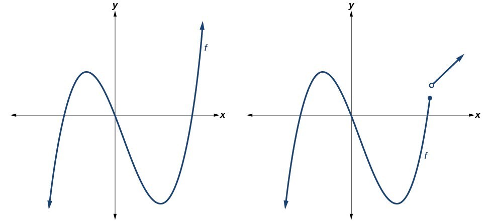
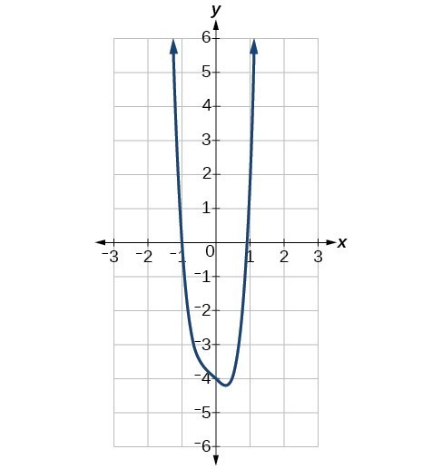
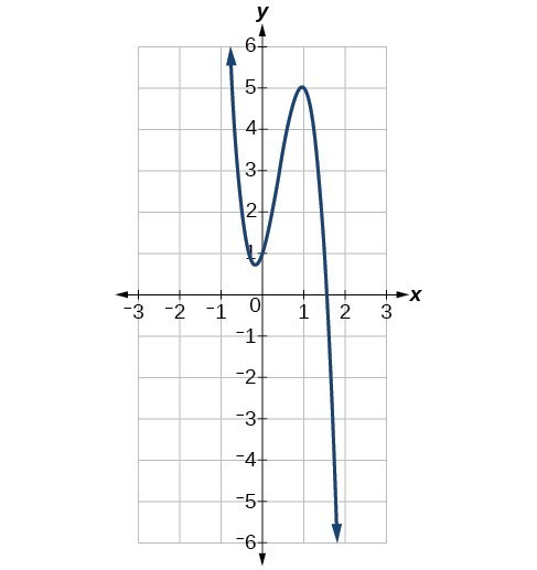
Polynomial functions of degree 2 or more have graphs that do not have sharp corners. These types of graphs are called smooth curves. Polynomial functions also display graphs that have no breaks. Curves with no breaks are called continuous. The figure below shows a graph that represents a polynomial function on the left, and a graph that represents a function that is not a polynomial on the right.
Example
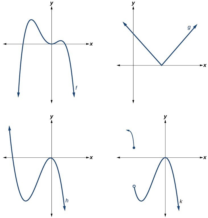
Which of the graphs below represents a polynomial function?
Identifying the shape of the graph of a polynomial function
Knowing the degree of a polynomial function is useful in helping us predict what it's graph will look like. Because the power of the leading term is the highest, that term will grow significantly faster than the other terms as x gets very large or very small, so its behavior will dominate the graph. For any polynomial, the graph of the polynomial will match the end behavior of the term of highest degree.
As an example we compare the outputs of a degree 2 polynomial and a degree 5 polynomial in the following table.
| x | \(f(x)=2x^2-2x+4\) | \(g(x)=x^5+2x^3-12x+3\) |
| 1 | 4 | 8 |
| 10 | 184 | 98117 |
| 100 | 19804 | 9998001197 |
| 1000 | 1998004 | 9999980000000000 |
As the inputs for both functions get larger, the degree 5 polynomial outputs get much larger than the degree 2 polynomial outputs. This is why we use the leading term to get a rough idea of the behavior of polynomial graphs.
There are two other important features of polynomials that influence the shape of it's graph. The first is whether the degree is even or odd, and the second is whether the leading term is negative.
Even degree polynomials
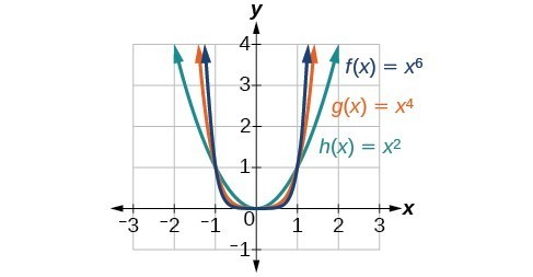
In the figure below, we show the graphs of \(f\left(x\right)={x}^{2},g\left(x\right)={x}^{4}\), and \( h\left(x\right)={x}^{6}\), which all have even degrees. Notice that these graphs have similar shapes, very much like that of a quadratic function. However, as the power increases, the graphs flatten somewhat near the origin and become steeper away from the origin.
Odd degree polynomials
The next figure shows the graphs of \(f\left(x\right)={x}^{3},g\left(x\right)={x}^{5}\), and \(h\left(x\right)={x}^{7}\), which are all odd degree functions. 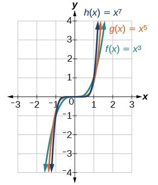
Notice that one arm of the graph points down and the other points up. This is because when your input is negative, you will get a negative output if the degree is odd. The following table of values shows this.
| x | \(f(x)=x^4\) | \(h(x)=x^5\) |
| -1 | 1 | -1 |
| -2 | 16 | -32 |
| -3 | 81 | -243 |
Example
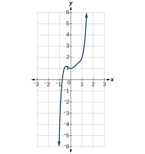
Identify whether graph represents a polynomial function that has a degree that is even or odd.
a)
b)
The sign of the leading term
What would happen if we changed the sign of the leading term of an even degree polynomial? For example, let's say that the leading term of a polynomial is \(-3x^4\). We will use a table of values to compare the outputs for a polynomial with leading term \(-3x^4\), and \(3x^4\).
| x | \(-3x^4\) | \(3x^4\) |
| -2 | -48 | 48 |
| -1 | -3 | 3 |
| 0 | 0 | 0 |
| 1 | -3 | 3 |
| 2 | -48 | 48 |
Plotting these points on a grid leads to this plot, the red points indicate a negative leading coefficient, and the blue points indicate a positive leading coefficient:
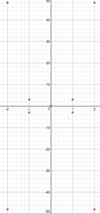
The negative sign creates a reflection of \(3x^4\) across the x-axis. The arms of a polynomial with a leading term of \(-3x^4\) will point down, whereas the arms of a polynomial with leading term \(3x^4\) will point up.
Example
Identify whether the leading term is positive or negative and whether the degree is even or odd for the following graphs of polynomial functions.
a)
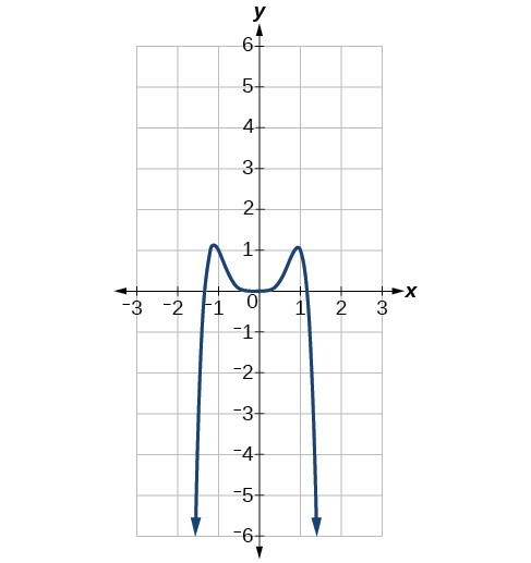
b)
Learning Objectives
- Add and subtract polynomial functions
- Multiply and divide polynomial functions
Just as we have performed algebraic operations on polynomials, we can do the same with polynomial functions. In this section we will show you how to perform algebraic operations on polynomial functions and introduce related notation.
The four basic operations on functions are adding, subtracting, multiplying, and dividing. The notation for these functions is as follows.
Addition \((f + g)(x) = f(x)+ g(x)\)
Subtraction \((f - g)(x)= f(x) - g(x)\)
Multiplication \((f \cdot g)(x)= f(x)g(x)\)
Division \(\frac{f}{g} (x) = \frac{f(x)}{g(x)}\)
We will focus on applying these operations to polynomial functions in this section.
Add and subtract polynomial functions
Adding and subtracting polynomial functions is the same as adding and subtracting polynomials. When you evaluate a sum or difference of functions, you can either evaluate first, or perform the operation on the functions first, as we will see. Our next examples describe the notation used to add and subtract polynomial functions.
Example
For \(f(x)=2x^3-5x+3\) and \(h(x)=x-5\),
Find the following:
\((f+h)(x)\) and \((h-f)(x)\)
In our next example we will evaluate a sum and difference of functions and show that you can get to the same result in one of two ways.
Example
For \(f(x)=2x^3-5x+3\) and \(h(x)=x-5\)
Evaluate: \((f+h)(2)\)
Show that you get the same result by
1)evaluating the functions first, then performing the indicated operation on the result and
2) performing the operation on the functions first, then evaluating the result
Multiply and divide polynomial functions
We saw that multiplying polynomials often required the use of the distributive property, and that the algebra of dividing polynomials could get messy fast! The same techniques can be used to multiply and divide polynomial functions. Additionally, the same idea applies to evaluating a product or quotient of functions as we discovered in the previous example. We can either evaluate the function and then perform the indicated operation, or vice-versa. You may already be thinking – it will be a lot less work to evaluate the polynomials and then divide the results!
Example
Given: \(g(t)=2t^3-t^2+7\) and \(f(t)=5t^2-3\)
Find: \((g \cdot f)(t)\), and evaluate \((g \cdot f)(-1)\)
In the next example we will divide polynomial functions and then evaluate the new function.
Example
Given \(p(x)=2x^2+x-15\) and \(r(x)=5x\)
Find \(\frac{p}{r}(x)\) and evaluate \(\frac{p}{r}(2)\)
Composite and Inverse Functions
Suppose we want to calculate how much it costs to heat a house on a particular day of the year. The cost to heat a house will depend on the average daily temperature, and in turn, the average daily temperature depends on the particular day of the year. Notice how we have just defined two relationships: The cost depends on the temperature, and the temperature depends on the day.

Figure 1
Using descriptive variables, we can notate these two functions. The function \(C\left(T\right)\) gives the cost \(C\) of heating a house for a given average daily temperature in \(T\) degrees Celsius. The function \(T\left(d\right)\) gives the average daily temperature on day \(d\) of the year. For any given day, \(\text{Cost}=C\left(T\left(d\right)\right)\) means that the cost depends on the temperature, which in turns depends on the day of the year. Thus, we can evaluate the cost function at the temperature \(T\left(d\right)\). For example, we could evaluate \(T\left(5\right)\) to determine the average daily temperature on the 5th day of the year. Then, we could evaluate the cost function at that temperature. We would write \(C\left(T\left(5\right)\right)\). By combining these two relationships into one function, we have performed function composition.
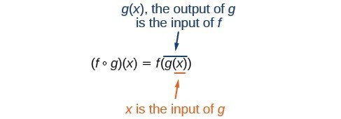
In the figure above, we read the left-hand side as "\(f\) composed with \(g\) at \(x,\)" and the right-hand side as "\(f\) of \(g\) of \(x.\)" The two sides of the equation have the same mathematical meaning and are equal. The open circle symbol \(\circ \) is called the composition operator.
It is also important to understand the order of operations in evaluating a composite function. We follow the usual convention with parentheses by starting with the innermost parentheses first, and then working to the outside.
Example
Using the functions provided, find \(f\left(g\left(x\right)\right)\) and \(g\left(f\left(x\right)\right)\).
\(f\left(x\right)=2x+1, \text{ } g\left(x\right)=3-x\)
In the following video you will see another example of how to find the composition of two functions.
Inverse Functions
An inverse function is a function for which the input of the original function becomes the output of the inverse function. This naturally leads to the output of the original function becoming the input of the inverse function. The reason we want to introduce inverse functions is because exponential and logarithmic functions are inverses of each other, and understanding this quality helps to make understanding logarithmic functions easier. And the reason we introduced composite functions is because you can verify, algebraically, whether two functions are inverses of each other by using a composition.
Given a function \(f\left(x\right)\), we represent its inverse as \({f}^{-1}\left(x\right)\), read as "\(f\) inverse of \(x.\)" The raised \(-1\) is part of the notation. It is not an exponent; it does not imply a power of \(-1\) . In other words, \({f}^{-1}\left(x\right)\) does not mean \(\frac{1}{f\left(x\right)}\) because \(\frac{1}{f\left(x\right)}\) is the reciprocal of \(f\) and not the inverse.
Just as zero does not have a reciprocal, some functions do not have inverses.
Inverse Function
For all functions, every input value has a single, unique output value. A one-to-one function is a function in which every output value has a single, unique input value.
For any one-to-one function \(f\left(x\right)=y\), a function \({f}^{-1}\left(x\right)\) is an inverse function of \(f\) if \({f}^{-1}\left(y\right)=x\).
The notation \({f}^{-1}\) is read "\(f\) inverse."; Like any other function, we can use any variable name as the input for \({f}^{-1}\), so we will often write \({f}^{-1}\left(x\right)\), which we read as "\(f\) inverse of \(x.\)"
Keep in mind that
\({f}^{-1}\left(x\right)\ne \frac{1}{f\left(x\right)}\)
and not all functions have inverses.
In our first example we will identify an inverse function from ordered pairs.
Example
If for a particular one-to-one function \(f\left(2\right)=4\) and \(f\left(5\right)=12\), what are the corresponding input and output values for the inverse function?
Analysis of the Solution
In the following video we show an example of finding corresponding input and output values given two ordered pairs from functions that are inverses.
How To: Given two functions \(f\left(x\right)\) and \(g\left(x\right)\), test whether the functions are inverses of each other.
- Substitute \(g(x)\) into \(f(x)\). The result must be x. \(f\left(g(x)\right)=x\)
- Substitute \(f(x)\) into \(g(x)\). The result must be x. \(g\left(f(x)\right)=x\)
If \(f(x)\) and \(g(x)\) are inverses, then \(f(x)=g^{-1}(x)\) and \(g(x)=f^{-1}(x)\)
In our next example we will test inverse relationships algebraically.
Example
If \(f\left(x\right)=x^2-3\), for \(x\ge0\) and \(g\left(x\right)=\sqrt{x+3}\), is g the inverse of f? Does \(g\) equal \({f}^{-1}?\)
In the following video we use algebra to determine if two functions are inverses.
We will show one more example of how to verify whether you have an inverse algebraically.
Example
If \(f\left(x\right)=\frac{1}{x+2}\) and \(g\left(x\right)=\frac{1}{x}-2\), is \(g\) the inverse of \(f\)? Does \(g\) equal \({f}^{-1}?\)
We will show one more example of how to use algebra to determine whether two functions are inverses of each other.
Domain and Range of a Function and It's Inverse
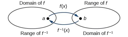
The outputs of the function \(f\) are the inputs to \({f}^{-1}\), so the range of \(f\) is also the domain of \({f}^{-1}\). Likewise, because the inputs to \(f\) are the outputs of \({f}^{-1}\), the domain of \(f\) is the range of \({f}^{-1}\). We can visualize the situation.
In many cases, if a function is not always one-to-one, we can still restrict the function to a part of its domain on which it is one-to-one. For example, we can make a restricted version of the square function \(f\left(x\right)={x}^{2}\) with its range limited to \(\left[0,\infty \right)\), which is a one-to-one function (it passes the horizontal line test) and which has an inverse (the square-root function).
Domain and Range of Inverse Functions
The range of a function \(f\left(x\right)\) is the domain of the inverse function \({f}^{-1}\left(x\right)\).
The domain of \(f\left(x\right)\) is the range of \({f}^{-1}\left(x\right)\).
In our last example we will define the domain and range of a function's inverse using a table of values, and evaluate the inverse at a specific value.
Example
A function \(f\left(t\right)\) is given below, showing distance in miles that a car has traveled in \(t\) minutes.
- Define the domain and range of the function and it's inverse.
- Find and interpret \({f}^{-1}\left(70\right)\).
| \(t\text{ (minutes)}\) | 30 | 50 | 70 | 90 |
| \(f\left(t\right)\text{ (miles)}\) | 20 | 40 | 60 | 70 |
Summary
Polynomial functions contain powers that are non-negative integers and coefficients that are real numbers. Polynomial functions can be added, subtracted, multiplied, and divided in the same way that polynomials can. It is often helpful to know how to identify the degree and leading coefficient of a polynomial function. To do this, follow these suggestions:
- Find the highest power of x to determine the degree function.
- Identify the term containing the highest power of x to find the leading term.
- Identify the coefficient of the leading term.
The inverse of a function can be defined for one-to-one functions. If a function is not one-to-one, it can be possible to restrict it's domain to make it so. The domain of a function will become the range of it's inverse. The range of a function will become the domain of it's inverse. Inverses can be verified using tabular data as well as algebraically.
Source: http://matcmath.org/press/3-5-polynomial-functions/
0 Response to "Inall Polynomial Functions Are Continuous and Reline"
Post a Comment